What are the measures of Variation

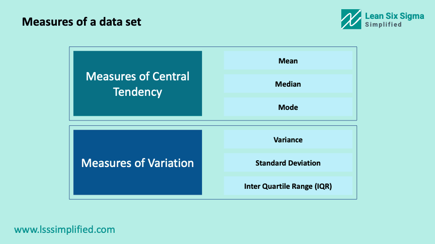
You can completely represent a data set by two key values, the measure of central tendency and measure of variation. You need both these measures to portray the true nature of the data.

In this post, we will look at what Variation means and what are the different measures of variation. Read on!

In the previous post, we discussed the measures of central tendency in details. We also spoke about what central tendency is and which measures you should use in what scenario. (Click on the link to read the post, opens in a new tab)

In this post, we will take a similar look at various measures of variation. We will look at Range, Interquartile range, Variance and Standard deviation. First, we will understand variation as a concept and why it is important to know the variation. Post that, we will see why using only central tendency is not enough for representing the data and why you should also use variation. We will then look at the measures of variation, their calculations, calculators and usage.

What is Variation?

Variation, or variability as it is sometimes referred to, is one of the summary statistics. It is used to represent the amount of spread or dispersion in the data set. It helps to understand how spread the values in the data set are. And how closer or farther each value is from the central tendency or midpoint of the data set.

Related Post : What is Measurement System Variation?

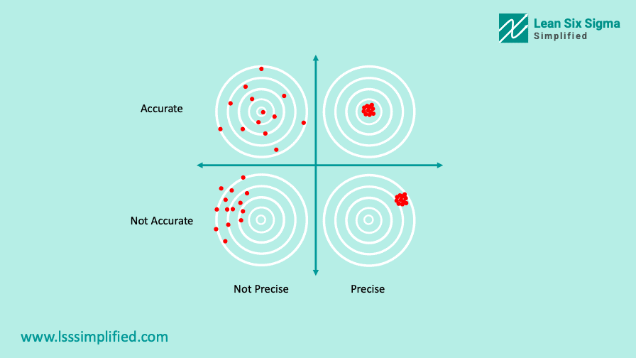
In order to understand what variation represents, think of an Archer doing target practice. She hits multiple arrows on the target. Once she is done shooting all the arrows, she draws a circle around the arrows such that all the arrows are within the circle itself. Think of variation as the radius of this circle. Bigger the circle, less precise the archer is. Smaller the circle, more precise the archer is.

Ideally, a good process should have minimum variation. Lower the variation, better the process. Lean Six Sigma projects essentially tend to reduce this variation from the processes to make them better.

There are multiple measures of variation in statistics. We will look at most relevant measures from Lean Sigma perspective. These are Range, Interquartile range, Variance and Standard Deviation.

However, before we delve into those, let us first understand the significance of measuring variation.

Significance of measuring variation

Most of the times, you would have noticed professionals quoting averages, or mean values of the data. They use this central tendency to summarize the data set. For example, the average score of a class or the average time taken to deliver your pizza.

Although the measure of central tendency is relevant, variation has more impact on the end customers. A parent will not care about the average score of the class if her child scores way below the average. You will not care about average delivery time of 20 minutes if your pizza comes after 40 minutes.

Usually, the end customer will expect consistency in delivery. If you know that a restaurant delivers pizza in 20 minutes, you will expect it in 20 minutes. And any delay, even of 5 or 10 minutes, will cause dissatisfaction. However, if you order from a restaurant which delivers pizza in 45 minutes, you will not expect it before 45 minutes. You will still be fine, or maybe even delighted, with a 40 minutes delivery.

Thus, measuring variation helps set up customer expectations from the process or product.

Measuring variation also helps you understand the extremes for your process. This further leads to identifying reasons behind such extremes and solve for it.

There will always be some variation in the processes, it’s inevitable. The issue arises at the extremes. And when the variation exceeds customer expectations or specifications.

Variation and Central Tendency

Let us now look at how variation plays a critical role in analyzing process performance.

There are 2 hypothetical transaction processing processes. Both of these processes have the same mean processing time of 20 minutes. The upper specification limits (maximum time expected by the customers) for both processes are also the same (25 minutes).

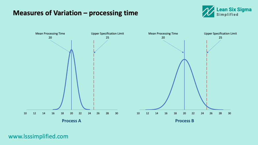
By comparing the mean processing time of these 2 processes, it looks like both are performing at the same levels. However, this alone is not enough information to make such a statement. We also need to look at the variation in these processes.

For the first process A, the lowest processing time was 16 minutes and the highest processing time was 24 minutes. For the second process, it was 12 minutes and 28 minutes respectively.

This information tells us that the spread for process A is much smaller than the spread for process B. It means, process A is more consistent in processing time as compared to process B. The variation in process A is less than the variation in process B.

From the customer expectations standpoint, process A will have higher customer satisfaction as it varies lesser than process B. And the probability of process A meeting the specification limits is higher than process B.

Now, we can definitely make the statement that process A is better than process B.

Central tendency alone does not provide complete information about process performance. It should always be looked at alongside variation in the process to get the complete picture.

Now that we understand what variation is and why understanding variation is important, let us look at the measures of variation.

Measure of Variation : Range

Range is the simplest measure of variation to understand and easiest to calculate.

Range is the difference between the largest and smallest data points or observations in the data set.

In our example above, process A has the maximum processing time of 24 minutes and minimum processing time of 16 minutes. Hence, range for process A is 24 – 16 = 8. Similarly, for process B, it is 28 – 12 = 16.

As you can see, the range is again higher for process B than for process A. Which means, variation in process B is higher than process A and hence, process A is a better process.

Disadvantages of Range as a measure of variation

Although range is fairly simple to understand and calculate, it does not give much information about the data set and the variation within. Since range depends entirely on the extreme values, it does not show how tightly or loosely the data is clustered around the center.

Since range depends only on the two extreme values, it is very prone to be influenced by outliers. If you have very high or low observations or values in your data set, which are not common data points, range calculation will still consider them.

For example, let us assume one of 15 transactions monitored from process A above, takes 50 minutes to process. This might be because of a special cause or a rare type of transaction, a one off instance. Range calculation will still consider such data points. Your range will change from 7 to 33.

This is important to understand because the process performance has not changed as such. The process will still keep performing between 16 and 24 minutes with an average time of 20 minutes. But Range will paint an entirely different picture!

Next thing we need to understand about range is its dependence on the sample size. If you have smaller sample size, the probability of extreme values getting picked up in the sample is low. This probability increases as you increase the sample size. Hence, the range will also increase with increasing sample size.

Range as a measure of variation is not useful when you have large sample size and when you have extreme values or outliers in your data sets. You should use it only when the sample size is small and free from outliers.

Measure of Variation : Interquartile Range (IQR)

We saw that the Range is the difference between the highest and lowest values in a data set. The Interquartile range, however, is the difference between the 1st and 3rd quartile of the data set.

First, we need to understand the Quartiles. We know that median divides the whole data set into 2 equal parts. (post arranging the data into ascending or descending order.) These 2 parts are 2 halves of the data. Please read the post on measures of central tendency to understand medians in details.

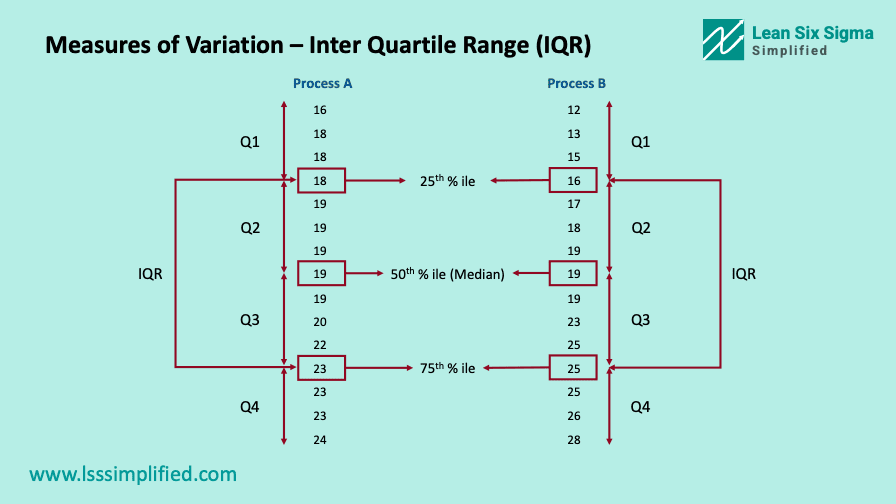
Similarly, each of these 2 halves can be further divided into 2 parts. Each of these parts is called a quartile, as it represents a quarter or 25% of the data set. These are denoted by Q1, Q2, Q3 and Q4, from low to high values.

Q1 is the lowest quartile which contains the lowest 25% of values from the data set. Q4 is the highest quartile which contains the highest 25% of values from the data set. Look at the below image for further understanding. I have divided the data from Process A and B from our previous example in quartiles.

In terms of percentiles, median is the 50th percentile.

• Q1 or first quartile lies between 0th and 25th percentile
• Q2 or second quartile between 25th to 50th percentile
• Q3 or third quartile between 50th and 75th percentile
• Q4 or forth quartile between 75th and 100th percentile of you data set

Interquartile Range or IQR is the difference between 75th and 25th percentile. It is the range of middle 50% of your data. It is the middle half of your data, after you arrange it in ascending or descending order.

IQR Calculation using Excel

First thing that you need to calculate IQR is the value of 25th and 75th percentile.

The excel formula to get these values is =PERCENTILE.EXC(array,k). Array is the range of cells where your data is stored and k is the percentile you wish to calculate. Remember, k has to be in terms of proportion ranging between 0 and 1, both excluded. For 25th percentile, k is 0.25.

Once you know the 75th and 25th percentile, the difference between these 2 values is IQR.

Interquartile Range (IQR) = percentile.exc(array,0.75) – percentile.exc(array,0.25)

IQR Calculation in MiniTab

Calculating IQR in MiniTab is fairly simple. Go to STAT > Basic Statistics > Display Descriptive Statistics from the MiniTab menu bar. A pop-up command box will appear.

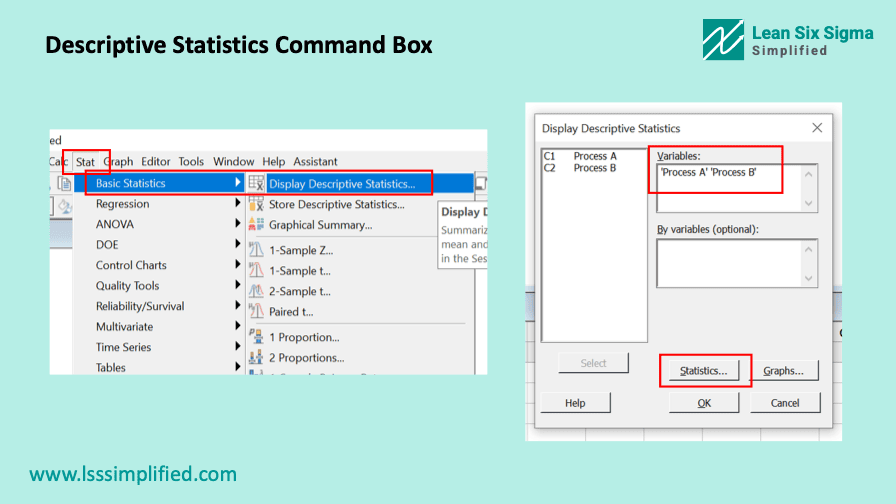
Select the column where you have the data stored as input for Variables and then click on Statistics button. Another pop up will appear as shown below.

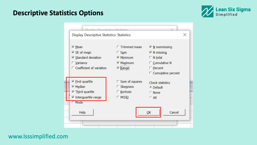
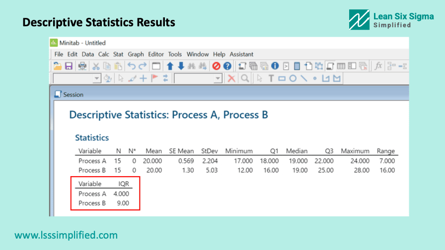
Tick the First Quartile, Third Quartile and Interquartile check-boxes. You can tick all other statistics as well which you wish to calculate for this data set. Once done, click on OK and run the test. You will get the results in the session window as shown below.

Semi Interquartile Range

A measure of variation related to Interquartile range is Semi Interquartile range. It is the Interquartile range divided by 2. If your data is symmetrically distributed, then the median will lie exactly at the middle of Q1 and Q3. That is between 25th and 75th percentile. In such cases, the the Semi Interquartile range will be equal to the difference between median and 25th percentile, as well as the difference between median and 75th percentile.

By the way, do check out the Certified Lean Six Sigma Black Belt Handbook – it is one of the most essential guide for anyone trying to get certified as LSS Black belt or in general wants to understand LSS and improve processes. – check it out here.

Advantages of Interquartile Range as a measure of variation

Interquartile range is a robust measure of variation. This is because it is not highly sensitive to the extreme values or outliers in your data set. Such extreme values or outliers have little impact on the IQR.

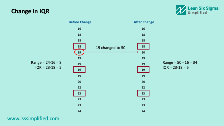
In our example above, I replaced the first value (19) for Process A by 50. We saw above that this changed the Range from 7 to 33. Below image shows the change in IQR due to this outlier. It changed from 4 to 5, a considerably lower change as compared to the change in Range.

Since it is not heavily impacted by outliers, it is an excellent measure for skewed distributions. Actually, for all distributions other than normal distribution.

Measure of Variation : Variance

Variance is a measure of variation that summarizes how far each of the observation is from the mean. It considers each data point in your data set in the calculation.

Statistically, Variance is defined as the average squared difference of values from the mean. It essentially summarizes the distances of each value in the data set from the mean.

Calculation of Variance of the data set depends on weather you are calculating it for the population, or for the sample to estimate it for the population.

Variance for a sample is denoted by s² and is calculated as per the below formula.

Here, X represents each individual value from the sample, μ represents sample mean and N represents the sample size. A sample usually has a tendency to underestimate the population variance. Hence, we use N-1 to correct for this underestimation.

Variance for the population is represented by σ² and is calculated as per the below formula.

Here, X represents each individual value from the population, μ represents the population mean and N represents the population size.

More often than not, we will not have visibility to the entire population. Hence, we calculate Variance for a sample from the population and estimate it for the population.

Variance Calculation

You can calculate Variance using MiniTab in the same was as described for calculation of IQR. Just ensure that you tick the check box for Variance and the results will show you the value for Variance.

In excel, you can use the formula =VAR.S(array) for sample variance calculation and =VAR.P(array) for population variance calculation.

These are easy and convenient ways to calculate the Variance of your data set. However, it is also important for all Lean Six Sigma practitioners to know how Variance is calculated manually. It is also important from the perspective of understanding Variance. So lets look at manual calculation of Variance as well.

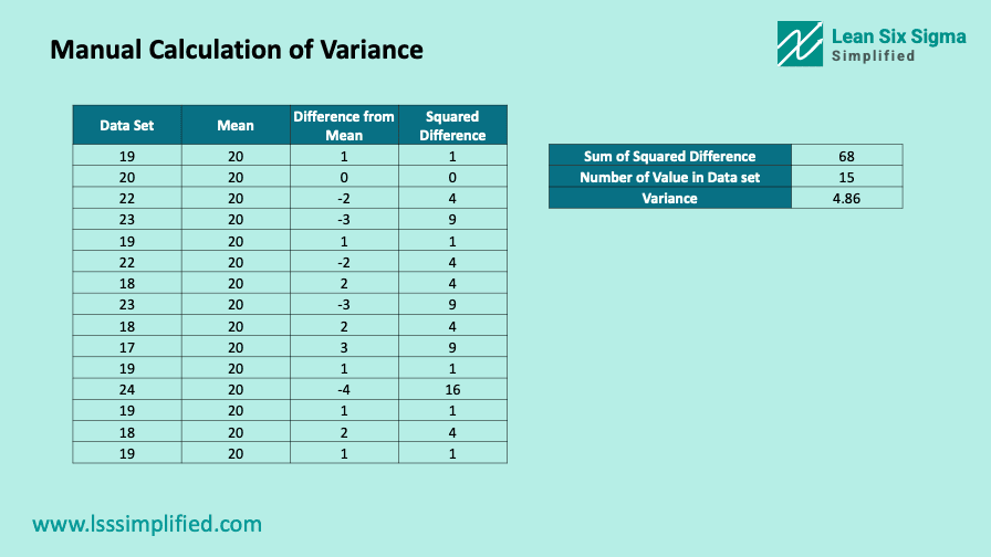
Steps to calculate Variance manually

• Step 1 : List down all the values from your data set in a single column. See “Data Set” column in the below image.
• Step 2 : Calculate the Mean of the data set and input in next column. See “Mean” column in the below image. Input this mean in each row for ease of calculations.
• Step 3 : Calculate the difference between the Mean and each value. Store in third column “Difference from Mean”.
• Step 4 : Take the square of the differences in third column. Store in the forth column “Squared difference”.
• Step 5 : Take the sum of all squared differences.
• Step 6 : Divide the sum by (N-1) where N is the count of values in your data set.

This is your variance. The data we have is a sample and hence we are using (N-1). If you have the data for whole population, use N instead of N-1.

Variance is an important statistical measure. Higher value of variance does mean higher variation in the process and vice versa. However, since it is a squared quantity, there is no intuitive way to compare this variance directly with the specific data values or the mean. Hence, although we calculate Variance as a measure of variation, we do not directly use it in our Lean Six Sigma projects.

Related Post : 12 Essential things you need to do in DEFINE stage of your DMAIC Project – Overview

So, to use this measure, we need to take the square root of this calculated Variance. That is where Standard Deviation comes into play.

Measure of Variation : Standard Deviation

Standard deviation is the square root of variance.

We discussed that Variance is in squared terms and not in the original unit of the data. Standard deviation solves this problem and returns the variance back to the original unit of the data. Thus, Standard Deviation can be used as a measure of variation which is easier to interpret and relate to the data set.

The same rule of measure of variation as discussed earlier apply for standard deviation as well. Lower the Standard deviation, better the process. Your Lean Six Sigma projects tends to reduce the standard deviation to improve processes.

Standard Deviation Calculation

As with Variance, Standard deviation calculation also differs for sample and population data. Standard deviation for sample is denoted by s and for sample is denoted by σ. As stated earlier, standard deviation is the square root of variance. Hence, to calculate standard deviation, you will first calculate Variance for the data set and take the square root.

You can also get the Standard deviation value using Minitab. Follow the same steps mentioned earlier for calculating IQR using ‘Display Descriptive Statistics’ option. Just ensure to tick the Standard deviation check box.

The standard deviation for our process A is 2.204 and for Process B is 5.03.

Standard deviation is a robust measure of variation for data which follows Normal distribution.

What does Standard Deviation tells us about the data?

I discussed the empirical rules of Standard deviation in my earlier post on Normal Distributions (opens in new tab). Please read this post to understand normal distribution and its properties.

Once we know the Standard Deviation of a data set, we can use it to determine the proportion of data values from the population, which fall between the mean and a particular number of standard deviations.

• 68.2% of the data values will always be between +/- 1 standard deviation from the mean
• 95.4% of the data values will always be between +/- 2 standard deviations from the mean
• 99.7% of the data values will always be between +/- 3 standard deviations from the mean

For Process A in our example, the mean is 20 and standard deviation is 2.204. Hence, we can make the below statements for Process A. (The assumption here is that the transaction time data for process A follows normal distribution.)

• 68.2% of the transactions from process A will be processed within 17.8 and 22.2 minutes (20 +/- σ)
• 95.4% of the transactions from process A will be processed within 15.6 and 24.41 minutes (20 +/- 2σ)
• 99.7% of the transactions from Process A will be processed within 13.4 and 26.6 minutes (20 +/- 3σ)

When to use which Measures of Variation

Now we know the measures of central tendency and the measures of variation. Below is the summary of which measures to use depending on the data that you have.

If you have normally distributed data, use Mean as measure of central tendency and Standard deviation as measure of variation.

If you have non-normally distributed data, use Median as measure of central tendency and Interquartile range as measure of variation.

That is all on measures of variation.

Do let me know your thoughts on measures of variation or if I missed to cover any aspect in this post in the comment section below. Appreciate your feedback.

Sachin Naik

Passionate about improving processes and systems | Lean Six Sigma practitioner, trainer and coach for 14+ years consulting giant corporations and fortune 500 companies on Operational Excellence | Start-up enthusiast | Change Management and Design Thinking student | Love to ride and drive

Read More about Sachin